Last
time we learned that DAX Query Plans are tree structures formatted as
indented text with each text line representing a single operator node in a tree.
A text line begins with an operator name followed by a colon and then properties
of the operator. Today we study the operator properties. You will see that for
the four types of operators, ScaLogOp, RelLogOp, LookupPhyOp, and IterPhyOp, each
type has a fixed set of common properties, and an individual operator may
contain extra properties to provide supplemental information. We’ll focus on the
semantics of the common properties in this post.
List of
Columns
In a DAX Query Plan, a list of columns is shown as a list of
comma-delimited column numbers in a pair of parentheses plus a list of
comma-delimited fully-qualified column names in another pair of parentheses, see
Figure 1. In a degenerate case, two pairs of empty parentheses, ()(), represent an empty list. Note that some properties, like
LookupCols
and IterCols, are not shown in the
plan when they contain no columns, but other properties, like DependOnCols and
RequiredCols, are always shown
even when their list of columns is empty.

Column numbers are helpful when you need to disambiguate two
separate references to the same column. When you execute Query 1 against the tabular
AdventureWorks database, the logical plan, shown
in Figure 2, assigns different numbers to column ‘Date’[Month]: number 1 refers to the column in the outer
table scan and number 2 refers to the column in the inner table scan. Column
numbers are not chosen to be globally unique, but rather unique within a local
context.
// Query 1
define measure 'Internet Sales'[Total Sales Amount] = Sum([Sales Amount])
evaluate
  calculatetable(
    addcolumns(
      values('Date'[Month]),           -- outer scan
      "YTD",
      calculate([Total Sales Amount],
          filter(
            All('Date'[Month]),        -- inner scan
            'Date'[Month]              -- refer to inner scan
            <=
            earlier('Date'[Month])     -- refer to outer scan
          )
      )
    ),
    'Date'[Calendar Year] = 2003
  )

Common
Properties of Logical Plan Nodes
Here are the properties common to all scalar logical
operators (ScaLogOp):
·
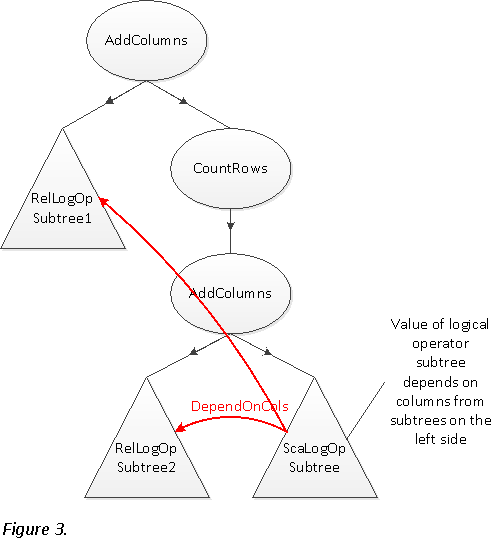
DependOnCols
Marks columns from the left-side
of a tree on which the current logical operator depends. The current operator
may return a different value for each distinct combination of values of DependOnCols. Some table scanning
functions, e.g. AddColumns and Filter, create a row context using its
left child subtree and then evaluate the value of its right child subtree in
this context. This creates a dependency of the right child subtree on some
columns from the left child subtree. DependOnCols
captures this correlation between the two sides of a tree. Figure 3 shows an
example where a ScaLogOp subtree on
the right depends on some columns from two RelLogOp
subtrees on the left. At the bottom level of a tree, DependOnCols are established by either an explicit reference to a
column on the left or by a leaf table scan that joins directly or indirectly
(through SetFilter arguments of Calculate
function) to columns on the left. DependOnCols
are then propagated up through intermediate parent nodes to the root node of the
right subtree. Since DAX automatic cross-table filtering rules can be tricky
sometimes, beginners can use this property to help them figure out whether
their measures have the correct dependencies on external row contexts.
·
Data type
One of the six data types DAX
supports. Values returned by the operator must be either of this data type or
be the BLANK value.
·
DominantValue
Captures the sparsity of a scalar
logical operator. When DominantValue
is NONE, the operator is dense, otherwise, it is sparse. When a scalar subtree
is sparse, DAX Formula Engine may pick a physical plan that can be orders of
magnitudes faster than a naïve physical plan. For example, if the predicate
child operator of a Filter operator
has a DominantValue of FALSE, DAX
Formula Engine can construct an iterator physical plan for the predicate
subtree that automatically skips large chunks of rows which would otherwise
return FALSE and be thrown away any way by the Filter operator. For users
coming from MDX background, this reminds them of the huge performance
difference between block mode vs. cell-by-cell mode. The technique to derive
the sparsity of a scalar subtree is very sophisticated and beyond the scope of
this post. It’s enough to know that a sparse scalar operator is the key to
great performance in many common query patterns.
Here are properties common to all relational logical
operators (RelLogOp):
·
DependOnCols
Identical to the same named
property of ScaLogOp. The current
operator may return a different table for each distinct combination of values
of DependOnCols.
·
Range of column numbers
Although a relation may contain
many columns in its heading, DAX Formula Engine is smart enough to derive the
minimal subset of columns, see RequiredCols
property, which are needed to answer a query. To save space, DAX Query Plan
does not list all columns in the relation header, instead, it assigns
continuous column numbers to all columns in the relation header and only shows
<beginning column name>-<ending column name> as a part of the plan.
Note that this property may be missing when a relation has no column at all.
·
RequiredCols
This is the union of DependOnCols and the subset of columns
from the relation header which are needed to answer a query. For example, when
you examine the logical plan, shown in Figure 4, which corresponds to Query 2,
you can see that only one column, [Sales Amount], among 129 columns is a
required column. In case you are wondering why ‘Internet Sales’ table has 129
columns, you can find the answer in one
of my earlier posts.
// Query 2
define measure 'Internet Sales'[Total Sales Amount] = Sum([Sales Amount])
evaluate row("x", [Total Sales Amount])

Common
Properties of Physical Plan Nodes
In a physical plan tree, an iterator operator supplies rows
of column values to other nodes. When those rows are fed to a lookup operator, it can return a scalar value
from each input row. When the rows are fed to another iterator operator, it can output any number of rows of its own columns for each input row. Therefore, both iterators and
lookups share the same input property, LookupCols, but they produce
different outputs. Let’s use the physical plan tree, shown in Figure 5, captured
from Query 1 to illustrate the common properties of physical operators.
Here are the properties common to all lookup physical
operators (LookupPhyOp):
·
LookupCols
Columns supplied by an iterator
whose values are used to calculate a scalar value. In Figure 5, lookup
operators 1 and 2 read their input values from iterator 3; their output values
are later on used by their parent operator, LessThanOrEqualTo,
to calculate a Boolean value.
·
Data type
One of the six data types DAX
supports. Values returned by the operator must be either of this data type or
be the BLANK value.
Here are the properties common to all iterator physical
operators (IterPhyOp):
·
LookupCols
Identical to the same named
property of LookupPhyOp. In Figure 5,
iterator 5, which doesn’t have the LookupCols
property, hence a pure iterator, supplies column 2 to iterator 4 as its LookupCols property which in turn
produces output column 1.
·
IterCols
Columns output by the iterator.
It is interesting to learn that a DAX iterator can be a pure
iterator, when it only has the IterCols property, or a table-valued function as in T-SQL Apply
operator when it has both LookupCols and IterCols
properties, or a pure row checker when it only has the LookupCols property. In the last
case, the iterator serves the purpose of removing unwanted rows from other
iterators.

For many DAX operators, common properties are all they offer.
But some DAX operators output additional properties to provide more information
about themselves. I am not going to go into details
about all those operator-specific properties today because it would drag this
blog on far too long. I’ll only describe the proprietary properties of one
physical operator Spool_IterOnly and postpone the
discussion of private properties of other operators in future blogs when we get
to study individual operators.
Special
Properties of Physical Operator Spool_IterOnly<>
Spool_IterOnly is a pure iterator that draws its rows from
an in-memory spool which is built through some other means. DAX Formula Engine
builds different flavors of in-memory spools, therefore Spool_IterOnly along with several
other physical operators built from spools put the name of the spool in a pair
of angle brackets <> as a part of their names. This is partly caused by
the fact that spools are not first class citizens in query plan trees as of SQL
Server 2012. As a result, some spool specific properties are added directly to
physical operators built on top of the spool. Below is one line I extracted from
Figure 5 with Spool_IterOnly specific
properties highlighted in bold face. They tell us that there are 12 records in
the spool and there are 240 key columns (most of which are compressed to 0 bit
hence record size is not as wide as it seems) and no value columns.
Spool_IterOnly<Spool>: IterPhyOp IterCols(1)('Date'[Month]) #Records=12 #KeyCols=240 #ValueCols=0
Summary
Today we studied properties of operator nodes in DAX Query
Plan trees. We have learned that some properties are common to all operators of
one type and some properties are specific to a particular operator. While I
described in details those common properties, I just cited one example of
operator specific properties. Now that we have covered the basics of DAX Query
Plans, we will be able to explore ways to take advantage of them to investigate
performance issues in future posts. When we run into a specific operator of
importance, I’ll explain its associated properties at that time.