The Logic behind the Magic of DAX Cross Table Filtering

Automatic cross filtering between columns of the same table or related tables is a very powerful feature of DAX. It allows a measure to evaluate to different values for different cells in a pivot table even though the DAX expression for the measure does not change. Filter context is the underlying mechanism that enables this magic behavior. But it is also a very tricky concept that even befuddles some DAX experts. Marco Russo and Alberto Ferrari have introduced DAX filter context in Chapter 6 of their book Microsoft PowerPivot for Excel 2010. Marco has also blogged about how Calculate function works. Recently I have run into many questions from advanced DAX users which tell me that people are still confused about how filter context works exactly. And this will be the subject of today’s post.

This post assumes that you already have basic knowledge about measures, row context, filter context, and DAX functions Calculate, Values, All, etc.

A level 200 pop quiz on DAX

If you think you already know how filter context works, let me ask you a couple of level 200 questions on DAX to see if you can explain the nuances of some DAX expressions. If you don’t feel like being challenged now, it is still beneficial to read the questions so you have some examples to better understand the following sections. The questions are based on the data model inside the publicly available sample PowerPivot workbook Contoso Samples DAX Formulas.xlsx. You can download the sample workbook to try out the formulas yourself if you want to, but it is not required to answer the questions.

Question #1.

People have heard that fact tables are automatically filtered by slices on dimension tables, but not the other way around, or in more general terms, if there is a relationship from table A to table B, A is automatically filtered by any slices on columns of B but B is not automatically filtered by any slices on columns of A. So if you select

DimProductSubcategory[ProductSubcategoryName] = “Air Conditioners”

on a pivot table slicer, measure

CountRows(DimProduct)

returns 62 as DimProduct is limited to air conditioners. On the other hand, if you select

DimProduct[ProductLabel] = “0101001”,

measure

CountRows(DimProductSubcategory)

returns 44 instead of just 1 although only a single product is selected. To filter DimProductSubcategory by the selected product label, you can define a measure as

Calculate(CountRows(DimProductSubcategory), DimProduct)

which returns 1. So it seems like when you explicitly add DimProduct as a setfilter argument of Calculate, DimProductSubcategory will be filtered by DimProduct. But if I define a measure as

Calculate(CountRows(DimProductSubcategory), Values(DimProduct[ProductLabel]))  

to explicitly add the column that I know having a slice from the pivot table to the Calculate function , the measure formula returns 44 again. So what makes setfilter expression DimProduct work but Values(DimProduct[ProductLabel]) not work even though the filter only comes from [ProductLabel] column? If you think you have to add foreign key DimProduct[ProductSubcategoryKey] to the filter context in order for DimProductSubcategory to be filtered by DimProduct, you can try

Calculate(CountRows(DimProductSubcategory), Values(DimProduct[ProductSubcategoryKey]))

but it still returns 44. If you have enough patience, you can use Values function to explicitly add all 33 columns in DimProduct one by one as setfilter arguments to Calculate function and you still will get 44 back. So what is the difference between table expression DimProduct and the enumeration of all 33 columns in that table?

Question #2.

There are 2556 records in DimDate table, therefore if you add a measure with expression

CountRows(DimDate)

to a pivot table without any filters, the measure value would be 2556. Now if you add a second measure with expression

Calculate(CountRows(DimDate), FactSales)

to the same pivot table, the measure value would be 1096 since DimDate table is filtered by FactSales table and only dates with sales records are included. But if you add a third measure with expression

Calculate(CountRows(DimDate), All(FactSales))

to the pivot table, the measure value becomes 2556 again. Since this pivot table has no filters anywhere, shouldn’t FactSales and All(FactSales) return the same table? Now add a fourth measure with expression

Calculate(CountRows(DimDate), Filter(All(FactSales), true))

to the pivot table, the measure value becomes 1096 again. All three setfilter arguments return exactly the same table, why would we get back different results?

With these questions in mind, let’s examine the logic foundation upon which the magic world of DAX is built. At the end of the post, you will be able to find a logical explanation to all these seemingly inconsistent results.

The expanded view of a DAX base table

The best way to understand DAX cross table filtering is to think of each base table as extended by its related tables. When a relationship is created from table A to table B, the new A, which is really A left outer join B, includes both columns of A and columns of B. So in DAX, a table reference FactSales really refers to

FastSales

LOJ DimProduct LOJ DimProductSubcategory LOJ DimProductCategory

LOJ DimStore LOJ DimGeography LOJ DimDate LOJ DimChannel LOJ DimPromotion,

where LOJ means left outer join. This interpretation makes it easy to understand some other DAX syntax. For example, in DAX expression

Filter(FactSales, Related(DimProduct[ProductLabel])  = “0101001”),

Related(DimProduct[ProductLabel])  refers to the value of column DimProduct[ProductLabel]  in the extended FactSales table. As a second example, DAX expression

AllExcept(FactSales, DimProduct[ProductLabel])

returns a table with all columns of extended FactSales table except for column DimProduct[ProductLabel].

Build initial filter context

DAX filter context is a stack of tables. At the beginning, the stack is empty. Given a pivot table, a filter context is initially populated by adding slicers and page filters. For each cell in a pivot table, current members of row labels and column labels also add filters to filter context. Other pivot table operations like visual totals add to initial filter context as well but I will keep things simple here. At this point, we have set up an initial filter context in which the measure expression of the current cell is to be evaluated.

Measure invocation

If SumOfSales is the name of a measure and Sum(Sales[Amount]) is its DAX formula, DAX expression

[SumOfSales]

is equivalent to

Calculate(Sum(Sales[Amount]))

 and DAX expression

[SumOfSales](Date[Year] = 2001, Store[Country] = “USA”)

is equivalent to

Calculate(Sum(Sales[Amount]), Date[Year] = 2001, Store[Country] = “USA”).

So the syntax sugar which makes a measure name look like a function name is just a clever way to add tables to filter context before evaluating the expression associated with the measure. Since invoking a measure implicitly calls Calculate, from now on I’ll just focus on Calculate function as the same rules apply equally to measures.

Add tables to filter context

Calculate function performs the following operations:

1.       Create a new filter context by cloning the existing one.

2.       Move current rows in the row context to the new filter context one by one and apply blocking semantics against all previous tables.

3.       Evaluate each setfilter argument in the old filter context and then add setfilter tables to the new filter context one by one and apply blocking semantics against all tables that exist in the new filter context before the first setfilter table is added.

4.       Evaluate the first argument in the newly constructed filter context.

If a new table is added to filter context and it has blocking semantics against some tables already in the filter context, the affected tables are checked one by one, all common columns with the new table are marked as blocked on the existing table.

Let’s look at an example. Assume the current filter context has two filters: one filter is Date[Year] = 2011, the other filter is Store[Country] = “Canada”. We want to evaluate the following expression in the context

AverageX(Distinct(Date[Month]), Calculate(Sum(Sales[Amount]), Store[Country] = “USA”)).

The first argument of AverageX sets a month in row context.  When it comes to Calculate, it first removes the month from row context and adds it to filter context, it does not block anything since there is no [Month] column in existing filters. Next Calculate adds Store[Country] = “USA” to filter context which blocks existing filter Store[Country] = “Canada”. When Sum(Sales[Amount]) is evaluated, Sales table is filtered by the current month in 2011 and stores in USA.

Targets of filter context

After so much effort populating and modifying a filter context, when will the filters be applied? In DAX, the filters in a filter context apply to following DAX table expressions:

1.       A table expression that is simply a table reference, such as FactSales.

2.       Values(Table[Column]).

3.       Distinct(Table[Column]).

In cases of 2 and 3, the Table is filtered by filter context and then distinct values of [Column] are extracted from the filtered table.

So if your expression is

Calculate(SumX(Filter(FactSales, [SalesQuantity] > 1000), [SalesAmount]), Date[Year] = 2011),

the filter context only restricts FactSales and has no effect whatsoever on other parts of the formula. If you image every DAX formula is represented as a tree of parent and child function calls, a filter context is built at the top or in the middle of the tree but takes effect at leaf level table nodes.

Note that DAX function Sum(T[C]) is just a shorthand for SumX(T, [C]), the same is true for other aggregation functions which take a single column reference as argument. Therefore the table in those aggregation functions is filtered by filter context.

Apply filters to a target table

Finally we have identified a target table and are ready to apply filters from filter context. For each filter table in the filter context, we check to see if there are any common columns between the target table and the unblocked columns of the filter table. If there is at least one common column, the target table is semi-joined with the filter table, or in SQL-like terms

SELECT *

FROM TargetTable AS t

WHERE EXISTS

(

SELECT *

FROM FilterTable AS f

WHERE t.CommonColumns = f.CommonColumns

)

Each filter table is applied to the target table independently, so the target table is filtered by all relevant filters.

All, AllExcept, AllNoBlankRow

So far I have said that each setfilter argument of Calculate function returns a table which is added to filter context. Well, that is true as long as the setfilter is not one of the All functions. The All functions should really be renamed as BlockColumns when they are used as setfilter arguments. If one of the All functions is used as the top-level function of setfilter, it only blocks common columns of earlier tables but does not add itself to filter context.

In all other places, including as a sub-expression of a setfilter but not at the top level, All functions behave like any other DAX table expressions and always return a table. One special feature of All functions is that the Table argument inside All(Table), All(Table[Column]), AllExcept(Table, …), AllNoBlankRow(Table), etc. is not filtered by the current filter context.

Pop quiz answers

Answer to question #1.

When the initial filter context contains column DimProduct[ProductLabel], table DimProductSubcategory is not filtered as it does not have that column.

Now look at the next formula

Calculate(CountRows(DimProductSubcategory), DimProduct).

The setfilter argument DimProduct is filtered by [ProductLabel], and then table DimProductSubcategory is filtered by table DimProduct since they both share the columns from table DimProductSubcategory and table DimProductCategory.

Move onto the next two formulas

Calculate(CountRows(DimProductSubcategory), Values(DimProduct[ProductLabel]))

Calculate(CountRows(DimProductSubcategory), Values(DimProduct[ProductSubcategoryKey]))

Both setfilter arguments are a single column table and the column comes from table DimProduct. Since table DimProductSubcategory does not have any column from DimProduct, it is not filtered by filter context. For the same reason, you can add any columns from DimProduct to the filter context and none of them would impact DimProductSubcategory.

Answer to question #2.

In the first formula

Calculate(CountRows(DimDate), FactSales)

Both table DimDate and table FactSales share columns from DimDate, so DimDate is filtered by FactSales.

In the second formula

Calculate(CountRows(DimDate), All(FactSales))

All(FactSales) blocks any columns from FactSales, but since the filter context is empty, it has no effect. When DimDate is evaluated, filter context is still empty.

In the third formula

Calculate(CountRows(DimDate), Filter(All(FactSales), true))

The All function is not at the top level of setfilter argument, table Filter(All(FactSales), true) is added to filter context, table DimDate is filtered by filter context for the same reason as in the first formula.

MDX Overwrite Semantics and Complex Attribute Relationship

The past month has been extremely busy for me so I didn’t get to write more blogs. Today we’ll resume the exploration of MDX calculation engine. In this post I am going to describe a common mistake made by people when writing MDX calculations that can be very hard to diagnose.

WARNING: The MDX overwrite behavior I am going to describe in this post applies to overwriting to a physical member or the [All] member. Overwriting to a calculated member has its own set of rules which are not covered here.

An Example

Let’s start with a simple example using Adventure Works DW 2008 database. First create a calculated measure, [m], that returns [Internet Sales Amount] for the first quarter of fiscal year 2004.

create member [Adventure Works].[Measures].[m] as

([Internet Sales Amount], [Date].[Fiscal].[Fiscal Quarter].[Q1 FY 2004])

Next send a query to check the value of [m].

select [m] on 0

from [Adventure Works]

m

$2,744,340.48

Now send another query calculating [m] but start with different calendar quarters.

select [m] on 0,

[Date].[Calendar].[Calendar Quarter].members on 1

from [Adventure Works]

	m
Q3 CY 2001	(null)
Q4 CY 2001	(null)
Q1 CY 2002	(null)
Q2 CY 2002	(null)
Q3 CY 2002	(null)
Q4 CY 2002	(null)
Q1 CY 2003	(null)
Q2 CY 2003	(null)
Q3 CY 2003	$2,744,340.48
Q4 CY 2003	(null)
Q1 CY 2004	(null)
Q2 CY 2004	(null)
Q3 CY 2004	(null)
Q4 CY 2006	(null)

Why don’t we see the value, $2,744,340.48, in all cells? Didn’t the MDX formula of [m] change whatever calendar quarter to the first quarter of fiscal year 2004? The answer lies in MDX overwrite semantics and attribute relationship of the [Date] dimension.

Examine the Example Based on MDX Overwrite Rules

Before we delve into details, let’s establish some terminologies first. MDX attribute relationship defines functional dependency between two attributes, e.g.

[Calendar Quarter] → [Calendar Semester] → [Calendar Year].

If A → B, we say B is related to A and A is relating to B. Therefore, [Calendar Semester] and [Calendar Year] are related attributes of [Calendar Quarter], and reversely [Calendar Quarter] and [Calendar Semester] are relating attributes of [Calendar Year].  On the other hand, [Fiscal Week] and [Calendar Quarter] are not related to each other.

Every MDX expression is evaluated in a context. In a simple case, the context includes the current cell which is defined by the current coordinates of all attributes in the cube. When an MDX expression, like ([Internet Sales Amount], [Date].[Calendar Year].[CY 2004]), overwrites the coordinates of some attributes to non-All members, it also overwrites the coordinates of all related and relating attributes. The following diagram illustrates how MDX overwrite semantics work when you set non-All slices to some attributes.

The common mistake I referred to at the beginning of the post is when people forget about the slices left over at the unrelated attributes. When dimension autoexists is applied and the new slices set by the MDX expression do not exist with the slices left over on the unrelated attributes, you end up with cells that don’t exist. Note that we don’t have this problem when there is only a simple linear attribute relationship defined on the dimension.

In case of a single linear relationship, all attributes in the dimension are always overwritten, either explicitly or implicitly, when any attribute is set to a non-All member. The problem arises only when there is a complex attribute relationship, one with tree-like structure.

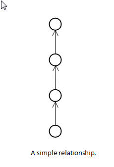
Going to back to the Adventure Works example, to calculate the value of any cell, an initial cell coordinate is set to a quarter from the [Calendar] hierarchy. Moreover, all related and relating attributes are set implicitly as well. See a simplified version of attribute relationship below. Every attribute in the diagram, except for [Month Name] is set to a slice that corresponds to a calendar quarter.

After applying the MDX expression associated with calculated measure [m], some attribute slices change to new ones, shown as colored boxes below, other attribute slices retain the previous values, shown as white boxes below.

You get a valid new cell only when the new slices correspond to the first quarter of fiscal year 2004 exist with the untouched old slices derived from the original calendar quarter; otherwise you get a cell that doesn’t exist hence a NULL value for the MDX formula. In this case only the third quarter of calendar year 2003 produces valid cell coordinates. To force setting the current coordinate to the first quarter of fiscal year 2004 regardless of the current calendar quarter, you have to explicitly overwrite all attributes related to the [Calendar] hierarchy like below:

create member [Adventure Works].[Measures].[m] as

(

      [Internet Sales Amount],

      [Date].[Fiscal].[Fiscal Quarter].[Q1 FY 2004],

      [Date].[Calendar].[All]

)

Official Rules

The above example is based on overwriting the current coordinate to a non-All member. But what about the other cases? Well, the following table lists all combinations of how overwriting one attribute can affect its related or relating attributes.

Assume A → B.

Explicit Overwrite	Result
A.All to A.All	B unaffected
A.x to A.All	B to B.All
A to A.x	B to Exists(B.members, A.x)
B.All to B.All	A to A.All
B.x to B.All	A to A.All
B to B.x	A to A.All

An implicit overwrite is when an attribute is moved because of an overwrite on a relating or related attribute. When an attribute is impacted by both an explicit overwrite and an implicit overwrite, the explicit takes precedence. Implicit overwrites do not overwrite related or relating attributes.

Parent Child Dimension

According to the overwrite rules discussed so far, overwriting the key attribute of a dimension to a non-All member should overwrite all other attributes in the dimension implicitly. But this does not work for parent child dimensions.

If you run query

with member measures.x as

(

      [Measures].[Amount],

      [Account].[Account].[Work in Process]

)

select x on 0,

([Account].[Account].[Raw Materials], [Account].[Account Number].[1162]) on 1

from [Adventure Works]

		x
Raw Materials	1162	(null)

You get back null result even though the calculation overwrites the key attribute [Account]. You have to explicitly overwrite [Account Number] attribute to get back the [Amount] for [Work in Process].

with member measures.x as

(

      [Measures].[Amount],

      [Account].[Account].[Work in Process],

      [Account].[Account Number].[All]

)

select x on 0,

([Account].[Account].[Raw Materials], [Account].[Account Number].[1162]) on 1

from [Adventure Works]

		x
Raw Materials	1162	$1,393,582.00

The official rule here is that:

Overwriting key attribute of parent child hierarchy does not overwrite other attributes except that of its parent.

Complex Relationships Are Very Common

Unless you define a single linear relationship for a dimension, you will end up with a complex relationship. Specifically, when there are more than two attributes in a dimension and you didn’t define any relationship, the default one is a tree-like relationship.

MDX Writeback with Custom Weight Expression

Users are likely to make the mistake we have discussed so far when the current cell coordinates contain many slices on numerous attributes. This is particularly true when it comes to MDX writeback with custom weight expression. When an MDX UPDATE CUBE statement is sent to Analysis Services, the desired result is allocated to leaf level nodes. So if you are writing a custom weight formula, the current context is always a leaf level cell with a slice on every regular attribute. If you are not careful overwriting all attributes in a dimension, your weight expression is likely to return NULL values and you won’t get the allocation you desired.

Conclusion

The complex rules of MDX overwrite semantics combined with a tree-like attribute relationship can easily lead to some very frustrating bugs in your MDX formula. You must make sure to overwrite slices on all attributes you don’t want to keep and preserve the slices on all attributes you do want to keep. Remember that the rules are different for parent child dimensions. If you have a simple tuple like MDX formula that returns unexpected NULLs, you should check whether you have violated the guidelines given in this blog post.

DAX Time Intelligence Functions

Time intelligence functions are an advanced feature of DAX. They are typically composite functions built on top of other more basic DAX features and have more stringent requirements for the structure of the underlying database. But since time related calculations are fundamental to almost all BI projects, early adopters of DAX started using the time intelligence functions almost immediately after the first release of DAX. Due to the advanced nature of these functions, questions naturally arise about how they work and why they work that way even when people managed to get the desired results.

Marius Dumitru, architect of AS engine team, gave the following recipe to users of time intelligence functions.

1.            Never use the datetime column from the fact table in time functions.

2.            Always create a separate Time table with contiguous dates (i.e. without missing day gaps in the date values).

3.            Create relationships between fact tables and the Time table.

4.            Make sure that relationships are based on a datetime column (and NOT based on another artificial key column).

5.            Make sure you have full years’ worth of data in the Time table. For instance, even though your transaction table may only have sales data up to May 2010, the Time table should have dates up to December 2010 (same goes for fiscal years).

6.            The datetime column in the Time table should be at day granularity (without fractions of a day).

In this post, I’ll expose more details behind the implementation of time intelligence functions to shed light on the rationale behind Marius’ advice. This post is meant to supplement online documentation of SQL Server 2008 R2. I will not cover basic usage examples of time intelligence functions in typical BI applications. DAX is a young functional language that evolves rapidly. What is covered here applies to SQL Server 2008 R2.

I assume you are already familiar with advanced DAX concepts such as row context, filter context, Calculate function, Values function, measures, etc. I’ll start with some common features across all time intelligence functions before I delve into individual functions.

The <dates> argument

All time intelligence functions have a special <dates> argument. FirstNonBlank and LastNonBlank operate on non-date/time columns but the conversion rules descibed below still apply. With the exception of DatesBetween and DatesInPeriod, the <dates> argument can be one of three forms:

1.       A reference to a date/time column.

2.       A table expression that returns a single column of date/time values.

3.       A boolean expression that defines a single-column table of date/time values.

Internally, all three forms are converted to a DAX table expression in the following fashion:

Format number	<dates> format	Internal table expression
1	T[C]	CalculateTable(Values(T[C]))
2	Single column table expression	As is
3	Well-formed scalar expression	Filter(All(T[C]), <scalar expression>)

What is a well-formed scalar expression? Vaguely speaking, it is a scalar expression that DAX engine can analyze and extract a fully qualified column reference to a date/time column. T[C] = Date(2011, 1, 17) is a well-formed expression as DAX engine can extract T[C] from it. T[C] * 2 is a well-formed expression for the same reason even though it is not a boolean expression DAX engine will cast it to boolean data type implicitly. Date(2011, 1, 17) is not a well-formed scalar expression as no column reference can be extracted from it.

Note that internally inserted CalculateTable in the first format automatically converts current row contexts to filter contexts. So

MaxX(Distinct(DimDate[CalendarYear]), OpeningBalanceYear([m], DimDate[Datekey]))

will give the maximum opening balance among all years, but

                MaxX(Distinct(DimDate[CalendarYear]), OpeningBalanceYear([m], Values(DimDate[Datekey])))

will not as the <dates> argument is in the second format hence not correlated to the current calendar year on the row context.

A special rule regarding datetime filter inside Calculate/CalculateTable

If a Calculate filter has a unique column that is of data type date/time, all previous filters on all columns from the table which contains this date/time column are removed. This hacky feature implies that

                Calculate(<expression>, <TI function>) = Calculate(<expression>, <TI function>, All(DateTable)).

This is the reason behind Marius’ recommendation #4. Let’s say you have some years on the pivot-table row and then you drag a measure which uses time-intelligence function DateAdd to show sales from the previous year. The author of the measure formula may not realize that DateAdd function only returns a single column of Datekey which overwrites existing filter on the same column. This special rule makes sure that the filter on the CalendarYear column, which comes from the pivot-table, is also removed so you get back the expected result. Without this special rule, Calculate(<expression>, <TI function>) would set days of the previous year on the Datekey column but leave the previous year as the filter on the CalendarYear column. The conflicting filters would have produced a blank result.

In PowerPivot v1, the only way to mark a column as unique is to create an incoming relationship to this column, hence Marius’ recommendation #3. You obviously also need a separate Date table in order to create a relationship.

In practice, people want to use integer keys to create relationship between Fact table and Date table. If you want to use time intelligence functions in that case, you must add All(DateTable) filter yourself to the measure expression.

In future versions of PowerPivot, users may be able to mark a date/time column as unique without creating an incoming relationship to the column. When that happens, recommendation #3 would no longer be needed.

Calendar

DAX engine creates an internal calendar data structure for each date/time column used in the time intelligence functions. The calendar contains a hierarchy of year-quarter-month-day. The minimum year and the maximum year in the calendar are determined by the actual dates in the date/time column. Internally, intermediate results are represented as arrays of days. So to represent January 2011, intermediate result would hold the 31 days in that month. Although a calendar contains all days in the years involved, it marks which days actually exist in the column. Calendar member functions return result days only if they are marked as exists. So if you have missing dates in the date/time column, they cannot be returned as a result of time intelligence functions.

When a calendar data structure is initially populated, it raises an error if two values from the date/time column correspond to the same day. So if you have a date/time column below the day granularity, it cannot be used in time intelligence functions.

Obviously calendar is an internal implementation detail which is subject to change in future releases of DAX. I mention it here to explain some of the limitations imposed on the current version of time intelligence functions. I’ll refer to calendar again when I discuss individual functions next.

Primitive time intelligence functions

As I mentioned at the beginning of the post, time intelligence functions are an advanced feature of DAX. They are built on top of other DAX features and functions, so there is nothing primitive about them. But many time-intelligence functions are composed from more basic time-intelligence functions which have their native implementations, I call the latter primitive ones.

FirstDate/LastDate/StartOfMonth/EndOfMonth/StartOfQuarter/EndOfQuarter/StartOfYear/EndOfYear return a table of a single column and a single row. They can be used anywhere a table expression or a scalar expression is needed due to implicit table to scalar cast.

As I described in the section on the <dates> argument, no matter which format the user uses, internally they are all converted to a table expression. From now on I will use <dates table> to denote the table expression equivalent to <dates>. I will use DimDate[Datekey] or simply [Datekey] to denote the date/time column extracted from <dates> expression.

FirstDate(<dates>)

LastDate(<dates>)

These two functions return a single column, single row table with values equivalent to

                MinX(<dates table>, [Datekey]), or

                MaxX(<dates table>, [Datekey]).

FirstNonBlank(<column>, <expression>)

LastNonBlank(<column>, <expression>)

These two functions are not pure time-intelligence functions as the first argument is not limited to <dates> as in all other time-intelligence functions. They are internally rewritten as

                Top1(Filter(<column table>, Not(IsBlank(<expression>)), [column]), and

                Bottom1(Filter(<column table>, Not(IsBlank(<expression>)), [column]) respectively.

Top1 and Bottom1 are internal functions similar to MinX and MaxX functions but support all DAX data types include boolean and string data types.
Note that <expression> is not automatically wrapped in Calculate, therefore,

                FirstNonBlank(DimDate[Datekey], Sum(FactSales[SalesAmount]))

does not give you what you want, but

                FirstNonBlank(DimDate[Datekey], Calculate(Sum(FactSales[SalesAmount])))

will produce the expected result.

StartOfMonth(<dates>)

StartOfQuarter(<dates>)

StartOfYear(<dates>, <year_end_date>)

Although not implemented this way, these functions first find FirstDate(<dates>), then jump to first day that exists in the same month/quarter/year.

EndOfMonth(<dates>)

EndOfQuarter(<dates>)

EndOfYear(<dates>, <year_end_date>)

Although not implemented this way, these functions first find LastDate(<dates>), then jump to the last day that exists in the same month/quarter/year.

DateAdd(<dates>, <number_of_intervals>, <interval>)

ParallelPeriod(<dates>, <number_of_intervals>, <interval>)

SamePeriodLastYear(<dates>)

SamePeriodLastYear(<dates>) is identical to DateAdd(<dates>, -1, Year).

Both DateAdd and ParallelPeriod invoke a function, Move, on the calendar object. The only difference is that ParallelPeriod requires the result days to fill an entire month/quarter/year, while DateAdd does not have this requirement.

Currently, DateAdd has a limitation that <dates table> must contain continuous days so that the result days can be continuous too.  We have this limitation because when you move all 28 days in February one month forward, like below,

                DateAdd(filter(All(DimDate[Datekey]), Year([Datekey]) = 2006 && Month([Datekey]) = 2), 1, Month)

you get back 31 days in March! As we mentioned in the section about Calendar, all intermediate results of time intelligence functions are represented as an array of days. So there is no difference between all days in February and February itself. But what if you have one day missing in the middle of February? Should we return one day missing in March or 27 days in March? This seems to be a tricky but less important question, so we left it undecided and raised an error instead.

The calendar object’s Move function is the most intelligent part of all time intelligence functions. It knows that moving both 3/30 and 3/31 one month forward end up on the same day 4/30. Internally it only moves by number of days or months, number of quarters or years is simply translated to corresponding number of months. Sometimes the Move function can be too smart for the user. When it moves a continuous range of days forward N months, it checks the start day and the end day of the range to see if you are moving whole months or just individual days. This works well when all days exist in the date/time column. But if you have missing days, the Move logic still tries to guess whether you are moving whole months based on days that exist, this may not be what you would expect, hence Marius’ recommendation #2.

DatesBetween(<dates>, <start_date>, <end_date>)

DatesInPeriod(<dates>, <start_date>, <number_of_intervals>, <interval>)

These two functions are different from the other time intelligence functions in that the <dates> argument can only be a fully-qualified column reference to a date/time column. Note that online document incorrectly states that the <dates> argument in DatesInPeriod can be any of the three formats.

Internally, both functions are rewritten as

                Filter(All(DimDate[Datekey]), DatesRange([Datekey], Earlier(<start_date>), Earlier(<end_date>))) or

                Filter(All(DimDate[Datekey]), DatesRange([Datekey], Earlier(<start_date>, Earlier(<number_of_intervals>), <interval>))

In the formulas above, Earlier is an internal extended version of the public Earlier function that evaluates an entire DAX expression by skipping the last row context. DatesRange is an internal boolean function that returns true if the value of the first argument falls within an interval. In case of DatesRange(<date_value>, <start_date>, <end_date>), the interval is defined as [start_date, end_date]. In case of DatesRange(<date_value>, <start_date>, <number_of_intervals>, <interval>), the interval is defined as [start_date, end_date) where end_date is calculated by calling the Move function on the calendar object, so it is a smart moveJ Note that since <number_of_intervals> can be a negative number, like when you move backwards in time, the interval specified by DatesInPeriod can be in the reverse order. DatesBetween does not allow reversed end points.

Also note that All(DimDate[Datekey]) implies that existing filter context does not apply to the date/time column, unlike when all other time intelligence functions use the name-pair syntax.

PreviousDay(<dates>)

PreviousMonth(<dates>)

PreviousQuarter(<dates>)

PreviousYear(<dates>, <year_end_date>)

Although not implemented this way, these function are equivalent to

FirstDate(DateAdd(<dates>, -1, Day)) in case of PreviousDay, or

DatesInPeriod(

<dates>,

StartOfMonth/StartOfQuarter/StartOfYear(

DateAdd(<dates>, -1, Month/Quarter/Year)

),

1,

Month/Quarter/Year

) in case of PreviousMonth/PreviousQuarter/PreviousYear.

NextDay(<dates>)

NextMonth(<dates>)

NextQuarter(<dates>)

NextYear(<dates>, <year_end_date>)

Although not implemented this way, these functions are equivalent to

LastDate(DateAdd(<dates>, 1, Day)) in case of NextDay, or

DatesInPeriod(

<dates>,

EndOfMonth/EndOfQuarter/EndOfYear(

DateAdd(<dates>, 1, Month/Quarter/Year)

),

-1,

Month/Quarter/Year

) in case NextMonth/NextQuarter/NextYear.

Composite time intelligence functions

The remaining time intelligence functions listed below are always internally rewritten using other time intelligence function.

DatesMTD(<dates>)

                DatesBetween(<dates>, StartOfMonth(LastDate(<dates>)), LastDate(<dates>))

DatesQTD(<dates>)

                DatesBetween(<dates>, StartOfQuarter(LastDate(<dates>)), LastDate(<dates>))

DatesYTD(<dates>, <year_end_date>)

                DatesBetween(<dates>, StartOfYear(LastDate(<dates>), <year_end_date>), LastDate(<dates>))

TotalMTD(<expression>, <dates>, <filter>)

                Calculate(<expression>, DatesMTD(<dates>), <filter>)

TotalQTD(<expression>, <dates>, <filter>)

                Calculate(<expression>, DatesQTD(<dates>), <filter>)

TotalYTD(<expression>, <dates>, <filter>, <year_end_date>)

                Calculate(<expression>, DatesYTD(<dates>, <year_end_date>), <filter>)           

OpeningBalanceMonth(<expression>, <dates>, <filter>)

                Calculate(<expression>, PreviousDay(StartOfMonth(<dates>)), filter)

OpeningBalanceQuarter(<expression>, <dates>, <filter>)

                Calculate(<expression>, PreviousDay(StartOfQuarter(<dates>)), filter)

OpeningBalanceYear(<expression>, <dates>, <filter>, <year_end_date>)

                Calculate(<expression>, PreviousDay(StartOfYear(<dates>, <year_end_date>)), filter)

ClosingBalanceMonth(<expression>, <dates>, <filter>)

                Calculate(<expression>, EndOfMonth(<dates>), <filter>)

ClosingBalanceQuarter(<expression>, <dates>, <filter>)

                Calculate(<expression>, EndOfQuarter(<dates>), <filter>)

ClosingBalanceYear(<expression>, <dates>, <filter>, <year_end_date>)

                Calculate(<expression>, EndOfYear(<dates>, <year_end_date>), <filter>)